insightcae-documentation
Automation of Simulation Workflows
Overview of the Project InsightCAE
Concept and Parts of the Project
The InsightCAE builds on top of available open-source engineering analysis tools (though closed-source tools could be used as well). The most used tool by far is the CFD software OpenFOAM.
For certain tasks, custom extensions to these tools are required. InsightCAE contains a selection of extensions, which are included in the distribution packages, when these are created.
The core of the project is the toolkit library. It contains the implementation of core classes in workflow management as the parameter set storage and tools and result set storage classes and handling tools. The toolkit library also maintains a list of available analysis modules, which is dynamically extensible by loadable add-ons.
Finally, on top of the toolkit library, custom analysis modules can be created. The InsightCAE base distribution contains a number of generic analysis modules as the “Numerical Wind Tunnel” module and some generic test case analyses like flat plate, channel flow, pipe flow and so on. These might serve as examples for custom implementations.
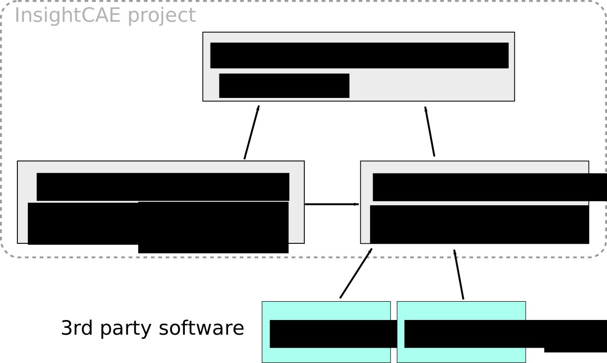 {#fig:insightcae-structure width=”75%”}
Terms and Definitions
Simulation App, Analysis
InsightCAE bundles tools to create automated simulation procedures. These procedures can be written in Python or C++. The term analysis, workflow module or Simulation App is used for such a procedure.
Actually, an analysis is like a function in programming: it gets input parameters, executed some actions (e.g. a numeric simulation) and returns a results data structure.
InsightCAE provides a GUI to edit the parameter sets and also tools to work with the result sets. E.g. convert the result set into a PDF report.
Parameter Set
The analysis modules need input data, i.e. parameters. All parameters for a module are grouped together in a parameter set. Parameter sets are stored in XML files in human readable format (extension *.ist). They can also be edited in a GUI editor (application workbench).
Many analysis modules need external files (like CAD data in STL or any other format). These files can simply be referred in a parameter set by their relative path (relative to the *.ist-file containing the reference) or absolute path. It is also possible to embed the external files into the XML file in an base64-encoded form. This simplifies transfer of analysis setup from one computer to another, e.g. for remote execution.
Result Set
The result of an analysis is returned in a result set. This is a hierarchical data structure which contains nodes like scalar values, charts, contour plots, images, tables or similar entities. It can be stored on disk in XML format. There is also a renderer which converts a result set into a PDF report.
Case Element
The setup of CFD-runs is put together from a number of so-called case elements. Each case element represents some functional feature. It might be a boundary condition or a turbulence model or something similar. A case element is not necessarily associated with a certain configuration file but can modify multiple configuration files of a CFD case configuration.
There is also an editor for composing OpenFOAM cases from the available case elements: the OpenFOAM Case Builder.
-
Solver extensions
-
OpenFOAM Case Builder
-
Workbench
Workflow Automation
Simulation Apps
Explanation of Building Bricks
Input: Parameter Sets
Parameter sets are a hierarchical collection of parameters. Parameters can be of different type, see the table below for a list.
A parameter set constitutes the full input data set for an analysis.
Beyond these primitive parameter types, there can be compounds, namely:
-
subset
a subdirectory in a parameter set
-
selectablesubset
a
subsetthat switches its content based on aselectionparameter -
array
an array of either a compound parameter or a primitve parameter
Throughout this manual and also e.g. in the command line parameters, the parameters are commonly specified in a file path-like format, where subsections are separated by slashes. For example, the parameter evaluateonly in the subsection run is meant by the expression run/evaluateonly.
For arrays elements, the index of the element is inserted after the array parameter name. For example, the parameter mesh/refinementZones/0/lx refers to the parameter lx inside the first array element of the array of subsections refinementZones in the subsection mesh.
| Type | Description |
|---|---|
double |
a scalar floating point value |
int |
an integer value |
bool |
a boolean value |
vector |
a 3-tuple of doubles |
string |
a simple text |
selection |
a selection from a predefined set |
path |
a file path, relative to the input file |
matrix |
a matrix with arbitrary number of rows and cols |
doublerange |
an array of double values |
Table: Available primitive parameter types in a parameter set {#tab:parameters}
Output: Results Sets
The output of an analysis is stored in a result set. It may contain elements like charts, images, tables, number etc. A result set can be saved to a XML file and/or rendered into a PDF report.
Analyses: the Simulation Procedure
The procedure of a simulation is contained in a so-called analyses or workflow module. You may think of it as an app for executing a certain type of simulation. It is essentially a program. Oftentimes, people create scripts or macros for speeding up their simulation workflows. The InsightCAE workflow modules serve a similar purpose, though the intention is to fully cover the whole simulation including all pre and post processing steps.
There is a GUI available which provides an editor for the input parameter set (see section 1.2.1). The GUI is also capable of displaying a 3D preview of the involved geometry and other elements, which are displayable. The analysis module is responsible of creating the 3D preview elements. Creation of the preview is optional and not every analysis module produces a preview.
The GUI also includes a viewer for the result set. From that viewer, the reports may be exported.
InsightCAE holds a runtime-extensible list of available analyses. This list can be extended at run time either by providing shared libraries containing more analysis modules or by python scripts.
The analyses can be programmed essentially in C++ or in Python. InsightCAE is essentially written in C++. Python wrappers for the relevant functions and objects are created using SWIG. So the API can also be accessed from Python.
If a new analysis shall be created, this parameter editing and result viewing infrastructure is easily reusable:
- The new analysis module just needs to provide the parameter set layout by returning the default parameter set (a parameter set filled with suitable default values),
- it has to provide a function for executing the analysis.
- This function needs to return a result set.
The analysis modules may group themselves into categories. This is used in the initial analysis creation dialog in the GUI.
Python Script
A python based analysis comprises a single dedicated python script file. The InsightCAE functions are included by an initial statement like from Insight.toolkit import *.
This script needs to define three standalone functions:
-
category()This functions returns a plain string with the category of the analysis. Multiple hierarchy levels are supported and have to be separated by slashes.
-
defaultParameters()This function shall return an object of type
ParameterSet, containing the default values of all the needed parameters. The user cannot add or delete parameters, just modify their values. So this defines the layout. -
executeAnalysis(parameters, workdir)This function finally runs the simulation. It gets an object of type
ParameterSet, containing all the input parameters and the stringworkdir, which contains the execution directory.
Upon loading, the InsightCAE base library searches in
-
$INSIGHT_GLOBALSHAREDDIRS/python_modulesand -
$INSIGHT_USERSHAREDDIRS/python_modules
for files named *.py. Each of these files will be loaded and their defined analyses will become available in the GUI and all other InsightCAE tools.
C++
In C++, a new analysis is derived from the common base class Analysis. The necessary functions have to be overridden. The new analysis should be put into a dedicated shared library.
Upon loading, the InsightCAE base library searches in
-
$INSIGHT_GLOBALSHAREDDIRS/modules.dand -
$INSIGHT_USERSHAREDDIRS/modules.d
for files named *.module. Each of these files has to contain a statement library <FILENAME>, where FILENAME is the name of the shared library file. These libraries will all be loaded and their defined analyses will become available in the GUI and all other InsightCAE tools.
Usage
GUI: workbench
The GUI for editing analysis parameters, run analyses and monitor their progress and to review the result sets is called workbench.
It can be started from the command line by executing
$ workbench
or from the global application menu.
The workbench can open and handle multiple analyses at a time. For each analysis, a sub window is opened (analysis form).
An analysis can either be created from scratch () or by opening an existing analysis input file (select in the menu).
The analysis form has three tabs. From left to right: the input parameter edit tab, the progress display tab and the result viewer tab.
Editing the Input Parameters
The parameter input tab is shown in figure 9. On the left, there is a tree view showing all the available parameters of the analysis. The font display style of the parameter entry denotes the importance of the parameter:
-
highlighted yellow background: these parameters have no reasonable default values and need to be changed for every case. The displayed default values are only chosen to demonstrate some functional value, e.g. for speeds or rpms. But for parameters like file names, for example, there is no reasonable default at all.
-
normal black text color: these parameters have reasonable default values, with which an analysis can be started. Though it is quite normal, that these parameters might need to be adapted from case to case.
-
dimmed gray text color: these parameters should normally be left at their default values. But it for rather rare special cases, it might become necessary to adapt them.
The parameters can be selected my mouse click and edited ().
Some analyses (this is optional) support a 3D preview of the configured case. When an analysis is loaded, which supports 3D preview, a 3D view and a 3D element tree appears right of the parameter edit column. All views in the Input tab are shown in a horizontal splitter and their width can be adapted by dragging the splitter handle between them. It is also possible to hide the 3D preview widgets by collapsing their width to zero using the splitter handle (This might also occur accidentally). The collapsing can be undone by locating the splitter handle of the collapsed widget and dragging it back to some non-zero width. The layout of the splitter is saved on program exit and restored on the next start.
Saving Parameters
Once all parameters are edited, the parameter set can be saved to a file. Very often, external files are referenced from a parameter set. Since it is also often necessary, to relocate parameter sets from one computer to another or between directories, InsightCAE parameter sets provide some special features which shall simplify relocation of parameter sets:
-
file paths are always stored as relative paths inside the parameter set file.
Even if the workbench editor displays an absolute path, the paths are made relative to the saving location of the parameter set file. It is still possible to insert absolute paths into a parameter set file. But when it is loaded and saved again, these will be made relative.
If a parameter set is moved around together with the files it references, they will be found, as long as they remain in the same relative location, e.g. side by side with the parameter file or in a sub directory.
-
external files can be embedded into the parameter file.
This is the preferred option, when parameter files shall be moved across computers. Upon saving, the files will be base-64 encoded (not compressed) and stored in the XML file. When the analysis is run, the files are extracted to a temporary location. The extraction is aware of the case, that different files with the same name might exist in different directories and extracts them to different locations. By default, the files are extracted to the system temporary location. When the InsightCAE application, which triggered the extraction of the parameter, exits, the files are deleted again from the temporary location. Note that this might not be achieved, if the application crashes.
Packing of external files can be enabled by checking or by checking the appropriate option in the “Save Parameters” dialog. Once, a parameter file was saved as packed or unpacked, the selection state is saved and used for all subsequent save operations.
Running the Analysis
With a properly edited parameter set, the analysis run can be started. This is achieved by clicking on the button “Run” on the right side or by selecting in the menu. This analysis form switches automatically to the “Run” tab (see figure 10). In the lower half, the log message are displayed. Sometimes, errors in an external program occur and are not correctly reported. It is therefore a good practice to watch the log messages for errors or warnings.
When the simulation solver runs, InsightCAE shows progress variables graphically. The plots are shown above the log widget. The number and meaning of the progress variables depend on the analysis conducted.
Especially for OpenFOAM-bases analyses, a number of quantities are extracted from solver output and forwarded to the GUI as progress variables:
-
continuity errors
-
equation residuals
-
forces
-
moments
-
execution time (per timestep)
Executing an Analysis on a Remote Host
Instead of running locally, an analysis can be executed on another computer: a Linux server, which is reachable via SSH, or a WSL (Windows Subsystem for Linux) distribution on the local Windows computer. The workbench stays the front end: parameters are edited locally, and progress, log messages and results are displayed as in a local run.
How a remote run works
On the remote host, the console program analyze (see section Console on Headless Computers: analyze) is started in server mode (analyze --server --port <port>). The workbench communicates with it through a small HTTP interface. A remote run passes through the following steps:
- Setting up the remote workspace: the remote working directory is created, if it does not exist (or a temporary one is created), and a free network port is determined on the remote host.
- Upload of the input file: the current parameter set is written as
param.istinto the remote working directory. External files should be embedded into the parameter set (see Saving Parameters), so that they are available on the remote side. - Launch of the remote analysis server:
analyzeis started in the background on the remote host. Its output is written toanalyze.login the remote working directory. - Establishing contact: the port of the remote server is made accessible on the local computer (for SSH hosts through an SSH tunnel; WSL ports are reachable directly), and the workbench waits until the server answers.
- Monitoring: the workbench polls the progress and log messages and displays them in the “Run” tab.
- Fetching the results: when the analysis has finished, the result set is transferred and loaded into the “Output” tab. Then the remote server is stopped.
- Download (optional): if “Download when finished” is checked, the remote working directory is copied into the local working directory (using
rsync). - Cleanup: a temporary remote working directory is removed.
If any of these steps fails, the steps performed so far are rolled back: the remote server process is terminated, including all its child processes (e.g. solvers), and a temporary remote directory is removed. The error message shows the reason, and in case of a failure of the remote server, also the last lines of its log file analyze.log.
Configuration of the remote hosts
The available remote hosts are defined in files called remoteservers.list. They are read from the InsightCAE share directories:
- the user-specific directory
~/.insight/share(on Windows%USERPROFILE%\.insight\share, or the directory given in the environment variableINSIGHT_USERSHAREDDIR), - the global directories (
/usr/share/insightor the directories listed in the environment variableINSIGHT_GLOBALSHAREDDIRS).
All files are combined. If the same label is defined in the user-specific and in a global file, the user-specific definition is used. The list can be edited in the workbench via Settings → Remote servers…. There, a host can also be marked as the preferred one.
The file has the following structure:
<root>
  <!-- Linux server, reachable via passwordless SSH -->
  <remoteServer label="cluster1" type="SSHLinux"
                host="cluster1.example.com" baseDirectory="/scratch/myuser" np="32"/>

  <!-- WSL distribution on the local Windows computer -->
  <remoteServer label="wsl" type="WSLLinux"
                distributionLabel="Ubuntu-22.04" baseDirectory="/home/myuser/runs"/>

  <preferredServer label="cluster1"/>
</root>
Attributes:
label: name, under which the host appears in the workbench,type:SSHLinuxorWSLLinux,host(SSH only): host name, as it is passed tossh(aliases from~/.ssh/configcan be used),distributionLabel(WSL only): name of the WSL distribution, as listed bywsl --list,baseDirectory: directory on the remote host, below which the temporary working directories are created,np(optional, default 1): number of processors available on the host.
For hosts, which are launched on demand (e.g. virtual machines), the attributes launchCommand and shutdownCommand can be given. They can also be entered in the server configuration dialog of the workbench (Settings → Remote servers…). These are executed locally, when the host is needed but not reachable, and when it is no longer needed, respectively. After the launch command, the workbench waits until the host becomes reachable (attribute launchTimeout in seconds, default 300). If it does not become reachable in time, the shutdown command is executed and the run fails with an error. A group of such hosts can be defined with an element remoteServerPool with the additional attributes maxSize and np. In this case, the placeholder %d in host, launchCommand and shutdownCommand is replaced by the instance number.
Note: in earlier versions, launchCommand, shutdownCommand and launchTimeout were called creationCommand, destructionCommand and creationTimeout. These names now have a different meaning (see below): existing server lists have to be adapted.
Cloud instances usually have to be created before they can be launched, and deleted when they are no longer needed. For this, the attributes creationCommand, destructionCommand and existenceCheckCommand can be given (all three or none):
existenceCheckCommandchecks, if the instance exists: an exit code of 0 means, it exists, any other exit code means, it does not exist.creationCommandis executed, when the host is needed, is not reachable and does not exist. Afterwards, the workbench waits until the host becomes reachable (launchTimeout). If it does not, thelaunchCommandis executed (if given) and the workbench waits again. If the host still does not become reachable, the created instance is disposed again.destructionCommanddeletes the instance. When disposing a running host, theshutdownCommandis executed before (if given).
In all five commands, the placeholders %{serverLabel} and %{host} are replaced by the label of the server and its host name, before the command is executed.
All commands can also be entered in the server configuration dialog of the workbench (Settings → Remote servers…). In this dialog, servers can also be launched (including the creation of their instance), shut down and disposed (Shutdown & Dispose). For a remote run, the execution panel offers the actions after completion: download of the results, removal of the remote directory, shutdown and disposal of the host.
Requirements on the remote host:
- the same version of InsightCAE is installed, and
analyzeis found in thePATHof a non-interactive login shell (bash -lc). This also applies to the helper scriptisPVFindPort.shand torsync. - SSH hosts: login via SSH without password (e.g. by public key authentication). On the local computer,
sshandrsyncneed to be available. - WSL: the distribution is installed and InsightCAE is installed inside it (the WSL setup wizard of InsightCAE can be used for this).
Selecting remote execution for an analysis
The execution location is configured in the analysis form by clicking “Setup…” in the “Execution” area. In the dialog “Setup Workspace”:
- the local working directory is selected (or left as temporary directory). For remote runs, a local directory is auto-created, if none is selected, but it is not removed afterwards.
- “Execute on remote host” is checked and the host is selected from the configured list.
- the remote working directory can be selected via “…”. If it is left at “(auto create)”, a temporary directory is created below the
baseDirectoryof the host, which is removed after the run.
If an analysis can not be executed on the local operating system (e.g. an OpenFOAM-based analysis on Windows), remote execution is preselected and can not be deselected.
The selected remote location is stored in the file meta.foam in the local working directory. When the analysis is opened again from this directory, the remote location is restored.
Controls during and after a remote run
Once remote execution is configured, the analysis form shows the host and the remote directory (“Run on remote host … in …”) and offers these buttons:
- “Run”: starts the remote run as described above.
- “Kill”: cancels the run. The analysis on the remote host is interrupted, the remote server is stopped and a temporary remote directory is removed.
- “Disconnect”: detaches the workbench from a running remote analysis without stopping it. The analysis continues on the remote host. The workbench may even be closed.
- “Resume”: reconnects to a remote analysis, which was disconnected before, and continues monitoring it (also after reopening the analysis from its working directory).
- “Download when finished”: if checked, the remote working directory is copied to the local working directory after the run has finished.
- “Upload to remote location” / “Download from remote location”: copy the contents of the working directory manually between the local and the remote side.
- “Remove remote”: deletes the remote working directory including its contents (only possible, while no remote run is active).
For OpenFOAM-based analyses, the buttons for triggering immediate output, for cleaning the case and for launching ParaView also work on the remote working directory. ParaView is then started as client-server pair (see “Launching Graphical Postprocessor ParaView” below).
Troubleshooting
- “The remote analysis server has exited during its startup” or “… has exited unexpectedly”: the message contains the last lines of
analyze.logfrom the remote working directory, including the exit code ofanalyze. Frequent reasons are:analyzenot found in thePATHof the remote login shell (“command not found”, exit code 127), or a different InsightCAE version on the remote host (unknown parameters in the input file). - “The log file … does not exist”: the server process was not started at all. Check, whether the remote working directory is writable and whether the remote host is reachable (
ssh <host> trueorwsl -d <distribution> --exec bash -lc true). - “Could not contact analysis server after launching it”: the server was started, but its port could not be reached, e.g. because of a broken SSH tunnel or a firewall.
Cancel a Simulation
To cancel a simulation run, click on the button “Kill” on the right side or by select in the menu.
Viewing the Results
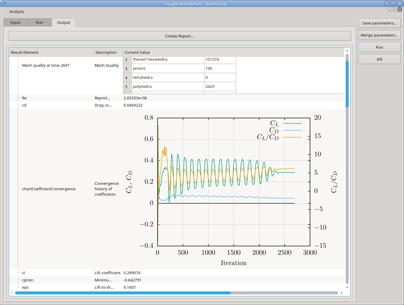
Once the simulation run is finished (that means that the solver has finished and that all post processing steps are done), a result set is created and loaded into the workbench. It is displayed in the “output” tab (see figure 11). The result set can be rendered into a report ().
Rendering Results into a Report
Modifying a Parameter
Creating a New Analysis
A new analysis is created by selecting in the menu . Then a new dialog appears, in which the list of available analyses is displayed (figure 8). The required analysis should be selected and confirmed by clicking “Ok”.
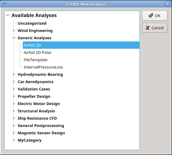 {#fig:workbench_new_analysis width=”50%”}
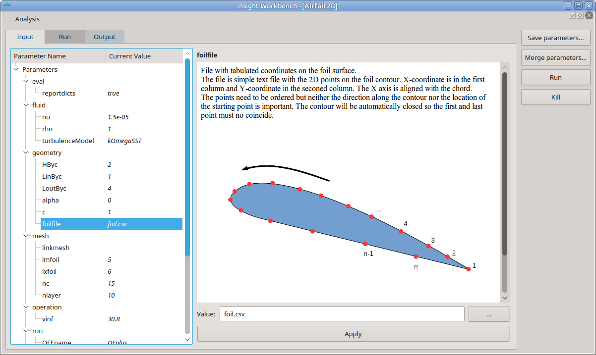 {#fig:workbench_parameters width=”100%”}
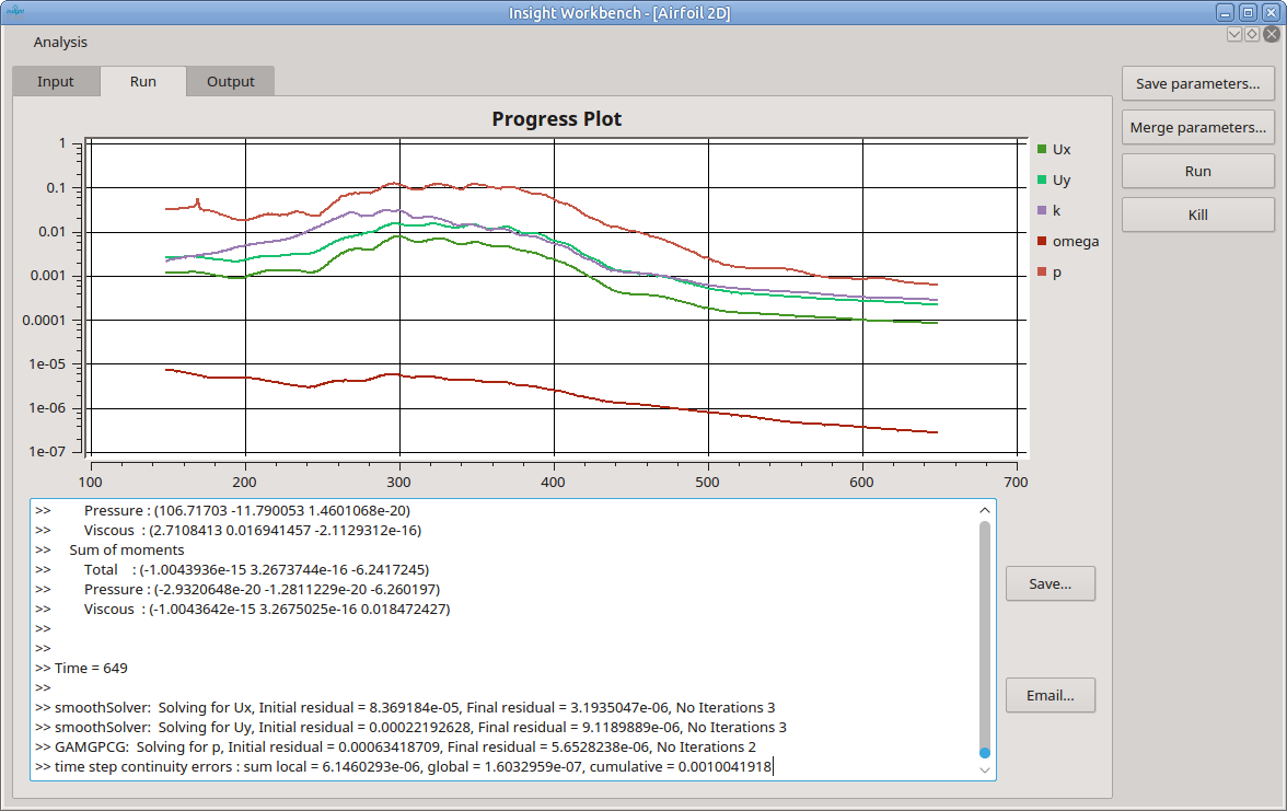 {#fig:workbench_progress width=”100%”}
 {#fig:workbench_result}
Special Features for OpenFOAM-based Simulation Apps
Simulation apps which are based on an OpenFOAM simulation provide some special features and also some implicit behavior and conventions which is documented in this section.
####### Restart Behavior
OpenFOAM-based simulations often run for a long time. It frequently appears that the simulation procedure is interrupted, either accidentally or intentional, and needs to be restarted.
There is no explicit function for a restart. It happens implicitly, when the analysis is re-launched in an existing working directory and some preconditions are met.
Depending on the state of the data, the behavior will be as follows:
-
if a mesh exists (in folder “constant/polyMesh/”) and a time directory exists (e.g. “0/”): it is assumed that the case is ready for execution and the solver will be restarted,
-
if only the mesh exists (“constant/polyMesh/”) and no time directory: mesh creation will be skipped. But all the dictionaries in
constant/andsystem/and field files in the initial time directory will be recreated.
Depending on where the interruption happened, the state might be inconsistent and invalid behavior might result. For example:
-
the interruption appeared within a meshing procedure which includes intermediate meshes → a mesh will be present but invalid
-
the interruption appeared during the field initialization → a time directory is present but the fields are invalid,
-
the interruption appeared during writing of a time directory → a time directory is present but invalid and the solver restart will fail.
If you are unsure about the validity of the case data, please consider to clean the case directory first and restart everything from the beginning (see 1.2.2.2).
####### Cleaning the Case Directory {#sec:cleancase}
When an OpenFOAM-based simulation run was performed, a number of directories and files are created in the working directory. If another run shall be performed and no restart is desired, then these directories and files need to be removed first. For this task, there is the standalone tool isofCleanCase, see section 3.4.
This tool can be launched in the selected workspace directory from within the GUI via the button “Clean” on the right side of the analysis form. Please see section 3.4 for details on the usage.
In some OpenFOAM-based simulation apps, auxiliary OpenFOAM case are created in subdirectories of the workspace directory. Currently, these can only be deleted or cleaned manually via a file manager and the command line tool isofCleanCase.
####### Performing only the Evaluation without Running the Solver {#sec:evaluateonly_workbench}
This is needed, if the solver was manually restarted, e.g. after manual changes of the numerical settings became necessary due to stability problems and ran until completion in the case directory which the corresponding InsightCAE simulation app has created.
It is then possible to execute only the evaluation part of the simulation app alone. This will not do any modifications to the simulation setup and it will not start any solver. To do this, the following is needed:
-
in the parameter set, set the switch
run/evaluateonlytotrue, -
set the working directory to the existing case directory, where the case was created (this will be done automatically, if an existing input file was opened),
-
then start the simulation by clicking the “Run” button.
Please note, that all parameters in the input file are assumed to match the simulation setup. No checks are done and there is no possibility for the Simulation app to restore them from an existing simulation folder. Thus it is up to the user to ensure validity.
####### Launching Graphical Postprocessor ParaView
To inspect the results of a OpenFOAM simulation beyond the figure which the InsightCAE simulation extracts automatically from the simulation case, the independent graphical postprocessor Paraview can be used.
It can be launched from the command line using a script as explained in 3.5.1.3.
Alternatively, this can be done also from the workbench. On the right border of the analysis form, there is a button labelled “ParaView”. For OpenFOAM-based simulation apps, this is enabled. Once it is pressed, Paraview will be launched in the selected working directory. If a local run is configured, it will just read the case from the selected working directory. If a remote run is selected, a client-server pair will be launched and the connection to the remote side is set up via SSH tunnels.
Console on Headless Computers: analyze
It is possible to launch an analysis from an existing input file (*.ist) without the graphical user interface in a batch mode. This is useful to integrate InsightCAE into workflows with other third-party software. The input file can be saved from the workbench (see 1.2.1.2) or created by a script or with any text editor.
To launch a simulation in batch mode, the executable analyze is available. It can be launched like this from the command line:
$ analyze inputfile.ist
The executable understands additional options. These are explanined in the following paragraphs.
Changing parameters
The values of parameters in the input file can be overridden from the command line by specifying an arbitrary number of the following parameters:
-
-b [ –bool ] arg
boolean variable assignment -
-l [ –selection ] arg
selection variable assignment -
-s [ –string ] arg
string variable assignment -
-p [ –path ] arg
path variable assignment -
-d [ –double ] arg
double variable assignment -
-v [ –vector ] arg
vector variable assignment -
-i [ –int ] arg
integer variable assignment
The argument arg for all these options has the form: path:value. The path is the file path-like specification of the parameter (see 1.1.1) and the value is appended to the name, separated by a colon. If any spaces are inside the value, e.g. when strings or path names are to be specified, then the entire arg should be set in qoutes at the command line. For example:
$ analyze --path "run/mapFrom:/a/path/with spaces" inputfile.ist
General Behaviour
The simulation working directory can be set explicitly by the parameter –workdir (short -w). The default is to use the current directory as the working directory.
The finally applied input parameter set is optionally saved to a file, when the file is specified with the parameter –savecfg (short -c).
Available Simulation Workflows
Numerical Wind Tunnel
Internal Pressure Loss
Working with Result Sets
The simulation apps produce result sets as output. These are collections of result elements. Result elements can be for example:
-
Plain values: scalar or vector
-
Matrices
-
Charts
-
Images
-
Files
-
Tables
Result sets can be
-
stored in a file (extension *.isr),
-
displayed with a viewer program. A viewer is embedded into the workbench (tab “output”) and a standalone viewer is available with the program
isResultTools -
or rendered into a PDF report.
-
In addition, with the
isResultTool, comparisons between multiple result sets or extraction of selected elements can be done.
Rendering of a Result Set
Result sets are displayed in the “output” tab of the workbench. When there are results displayed, those can be rendered or saved into an ISR file by selecting
Whether a PDF report is rendered or a ISR file is written, depends on the file extension which is entered in the file dialog.
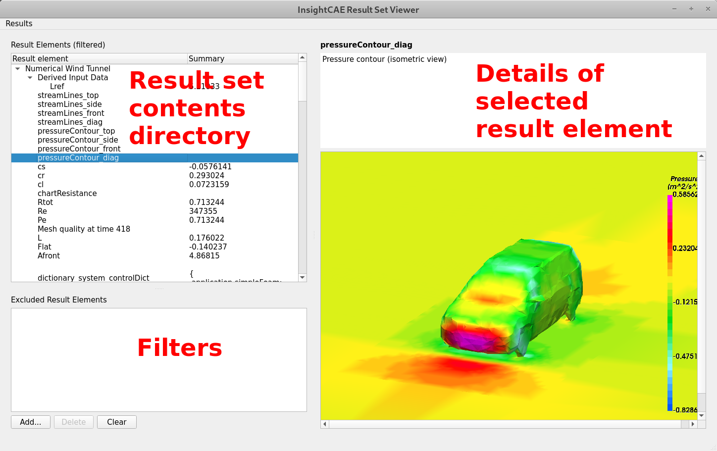
A report can also be rendered from a ISR file on disk. Therefore the executable isResultTool exists. Once the program is started, select in the menu and select the ISR file in the file selection dialog. The result elements are then shown in the tree view on the left side of the window (12b). To render the result elements into a PDF, select in the menu and enter a file path to the desired output PDF file. Optionally, some result set elements can be omitted from the PDF rendering by applying filters, see 2.0.0.2.
 {#fig:isresulttoolmainwindow width=”100%”}
Alternatively, the tool isResultTool can be executed with the command line argument –render:
$ isResultTool --render savedResultset.isr
Applying Filters during Rendering
A set of filters can be defined to render a report with some result elements excluded. A filter is just a path-like text which represents the location of the result element in the result set hierarchy. The concept is very similar to the specification of parameters, see section 1.1.1 above. Every result element, where the label path matches one of the filter expressions, is excluded. The filter expressions, which are already defined, are shown in the list in the bottom left corner of the Result Set Viewer window, see figure 12a. The result set content directory, which is displayed in figure 12b, shows the result set contents with all filters already applied.
To add filter expressions, click on the button “Add...”. The result element paths to filter out can be directly typed into the text field, one per line. Instead of typing, result elements can be select from the full content of the result set after clicking the “...” button.
By default, a direct match of the entered text with the result element path is required. Alternatively, the text entered in the input field can be treated as a regular expression[^5][^6]. If a regular expression was entered and shall be treated as such, the selection below the input field has to be changed to “regular expression”.
Once a set of filter expressions is defined, it can saved to a file by selecting.
Vice versa, a previously saved set of filter expressions can be loaded by .
When the a report is rendered or saved into a ISR file, there is a switch on the bottom of the file dialog (“Save filtered result set”). This is by default checked. If this is unchecked, the filter is skipped and the full report is rendered or saved.
Supporting Simulations with OpenFOAM
Case Setup GUI: isofCaseBuilder
Execution Monitor GUI: isofExecutionManager
Tabular Output Data Plot: isofPlotTabular
Clean OpenFOAM Case Directories: isofCleanCase
Common Tasks in the Context of OpenFOAM Simulations
Controlling and Checking Running OpenFOAM Case Which Were Generated by InsightCAE
OpenFOAM cases which were generated by InsightCAE are enhanced with a number of additional features. These are utilized by the workbench frontend but can also be used to modify cases manually.
####### Trigger Output Independently from the Configured Output Interval {#par:trigger_output_of}
[]{#par:wnow label=”par:wnow”}
The solver monitors the files in its case directory. If it finds a file named wnow, immediate output is triggered and this signal file is removed by the solver.
This feature can be used to inspect the solution at any time while the solver is running using Paraview.
The file can e.g. created from the terminal:
$ touch wnow
Note: you might need to change to working directory to the case directory first.
####### Trigger Immediate Output and Stop Solver Afterwards Without Raising an Error {#par:wnowandstop}
The solver monitors the files in its case directory. If it finds a file named wnowandstop, immediate output is triggered, this signal file is removed by the solver and the solvers.
This feature can be used e.g. to gracefully and a solver run which is converged and the convergence is recognized by the user but not yet by the convergence monitoring feature of InsightCAE.
The file can e.g. created from the terminal:
$ touch wnowandstop
Note: you might need to change to working directory to the case directory first.
####### Inspecting a Running Case Using Paraview {#par:isPVpy}
Some of the relevant numerical figures of a case are displayed in live updated charts in the GUI. But it is a very good habit to check the mesh and also the solution as soon as possible and well before valuable computing resource are wasted to compute inadequate solutions on bad meshes. If problems with the mesh or the solutions become obvious, it is possible to stop the analysis (e.g. by the “Kill” button in the workbench or by pressing CTRL+C in the terminal, where the analyze command line tool is running) and revise the settings.
The OpenFOAM cases can be loaded into Paraview as soon as they were created by one of the InsightCAE modules. It is perfectly possible to do this while the solver is running. It is also possible to trigger extra output if it is not yet available (see first paragraph of this section).
-
When output[^7] is there, Paravie w is best launched by InsightCAE’s wrapper script
isPV.py:$ isPV.pyNote: you might need to change to working directory to the case directory first.
-
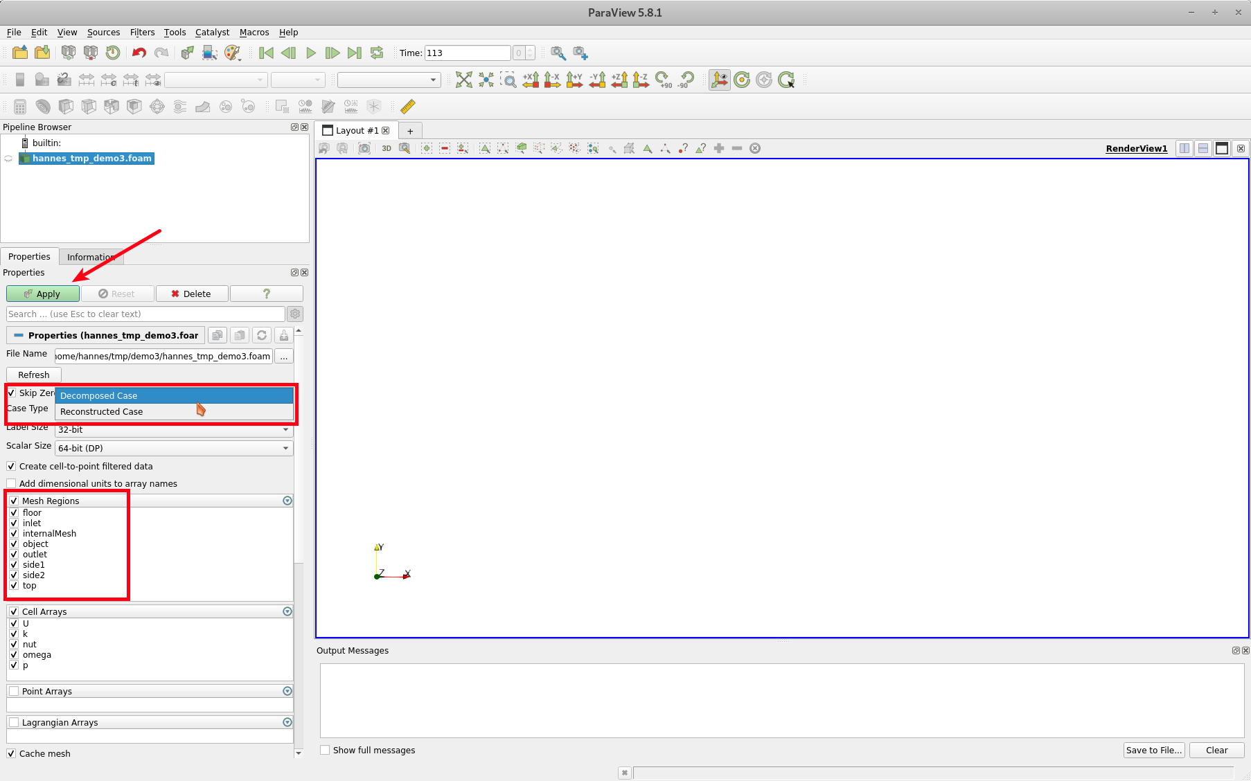
The wrapper automatically inserts the OpenFOAM case reader source into Paraviews’ visualization pipeline. You should consider the following settings:
-
Select at least all the mesh regions, which you would like to inspect. You can later filter out subsets of mesh regions. So it is ok, to select all.
-
Select the case type: either
-
“Reconstructed Case”, if you performed a serial run or if the output has been already reconstructed from the processor directories (usually done for the last time step during the evaluation step)
-
“Decomposed Case”, if you want to monitor a parallel run.
-
When all settings are right, click on “Apply”.
 {width=”75%”}
 -
-
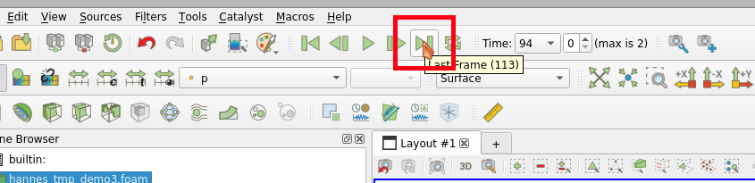
Next, jump to the latest time step:
 {width=”75%”}
 -
Now, the scene can be set up using all the Paraview filters[^8].
Often, fields on boundary regions (e.g. walls) are of interest. These can be extracted using the “Extract Block” filter. To apply this filter, select from the menu . Make sure that the OpenFOAM case source is selected in the pipeline browser when the filter is added. When all the boundaries of interest are selected, click on “Apply”.
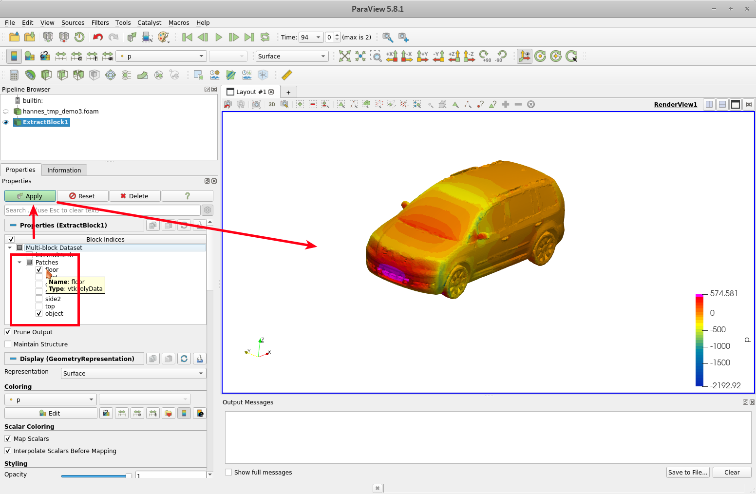 {width=”75%”}
Meshing
####### Extraction of Feature Edges from STL Geometries
Features edges can be extracted automatically from STLs. They are usually found by looking at the angle between neighbouring triangular facets. This methods is usually automatically applied either in snapphyHexMesh itself or within InsightCAE’s workflows. This method works nicely for edges between planar surfaces. Though it fails e.g. for rounded edges like leading and trailing edges of propellers and foils. In such cases, it is required to extract feature edges manually and feed them into the meshing process.
Here, it is described how to extract feature curves using the open source software Blender[^9]. The following steps are required:
-
Import the geometry into Blender
select in menu
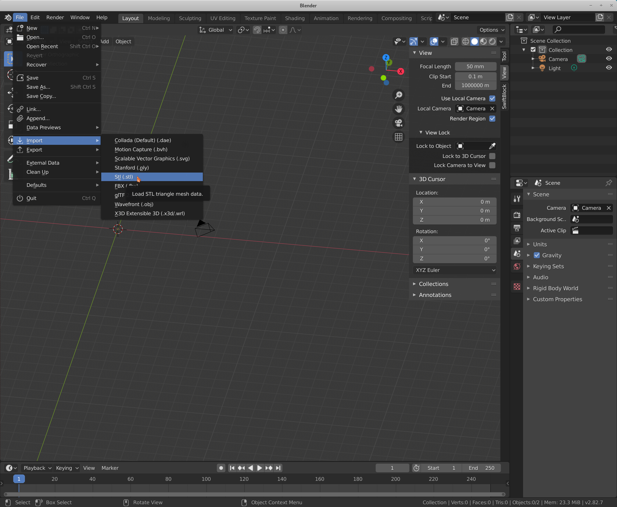 {width=”75%”}
 -
select the STL file
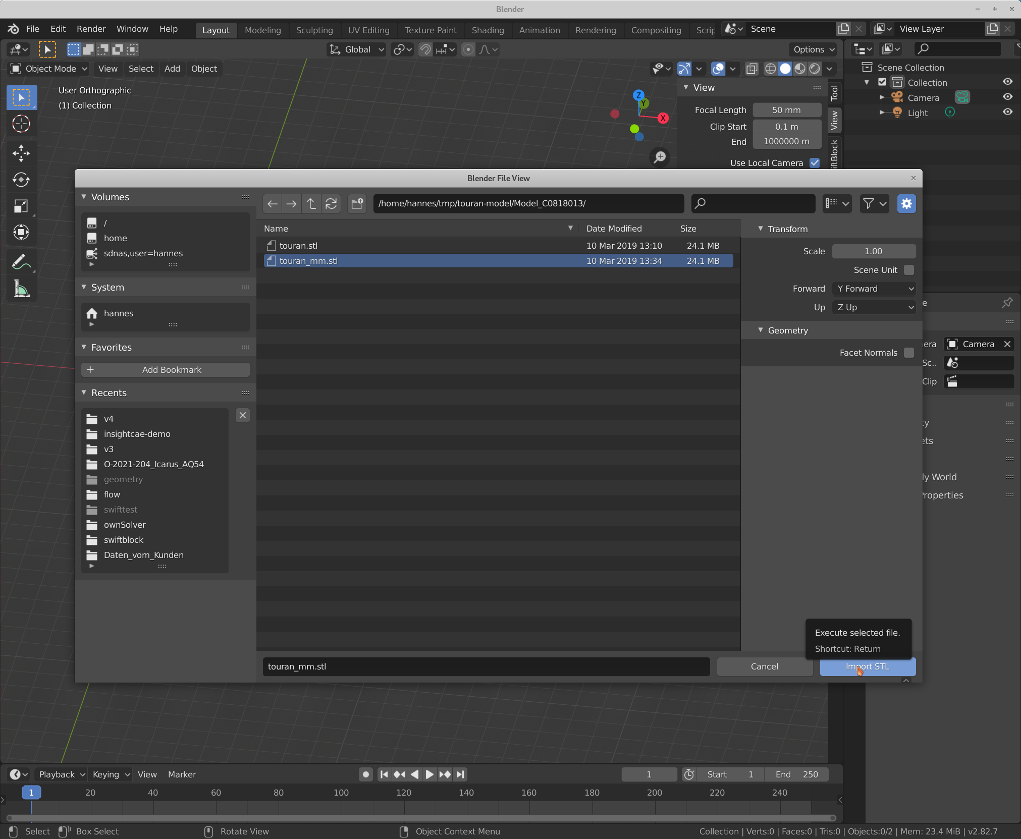 {width=”75%”}
 -
make sure, the object is selected (orange line around the selected object is displayed)
Objects can be selected by left click them with mouse.
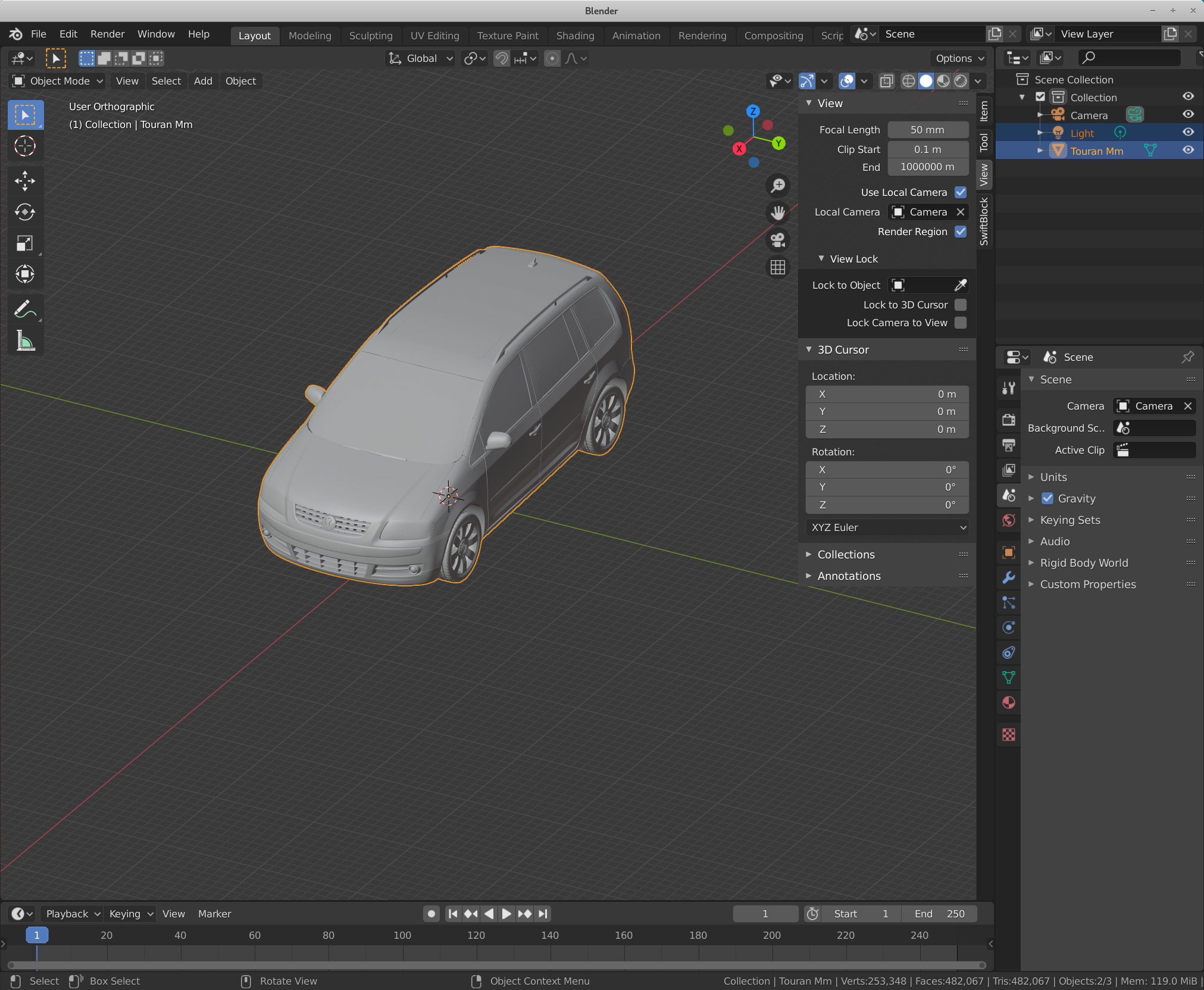 {width=”75%”}
 -
switch to “Edit Mode”, either by pressing the “Tab” key or by selecting the mode in the combo box in the upper left corner.
Next, switch to edge selection mode (second button right from the edit mode combo box)
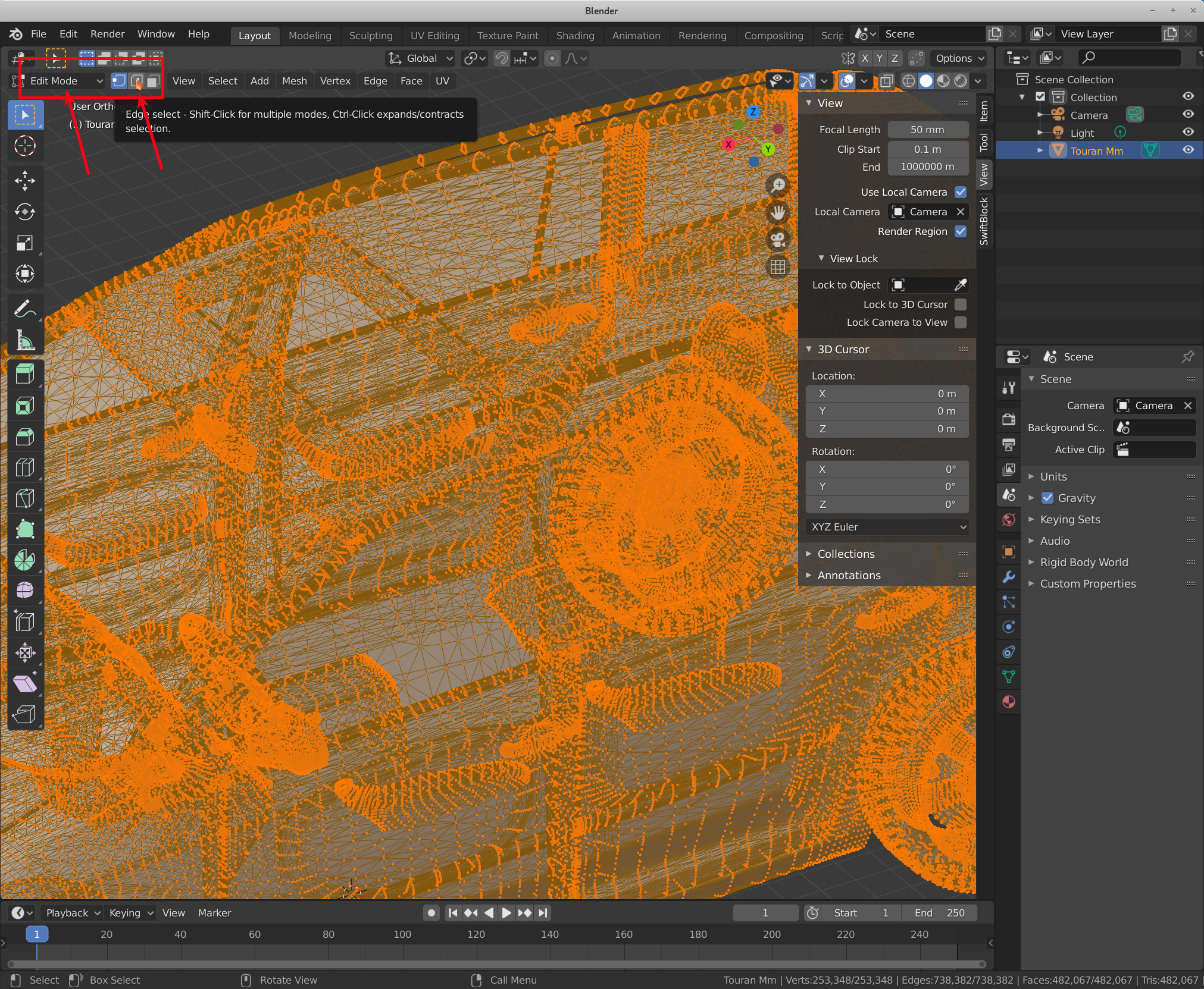 {width=”75%”}
In this example, we want to select a line (chain of edges) along the left roof rail.
-
zoom into the location of the beginning of the line []{#pt:begin_sel label=”pt:begin_sel”}
select the first edge with a left click on it.
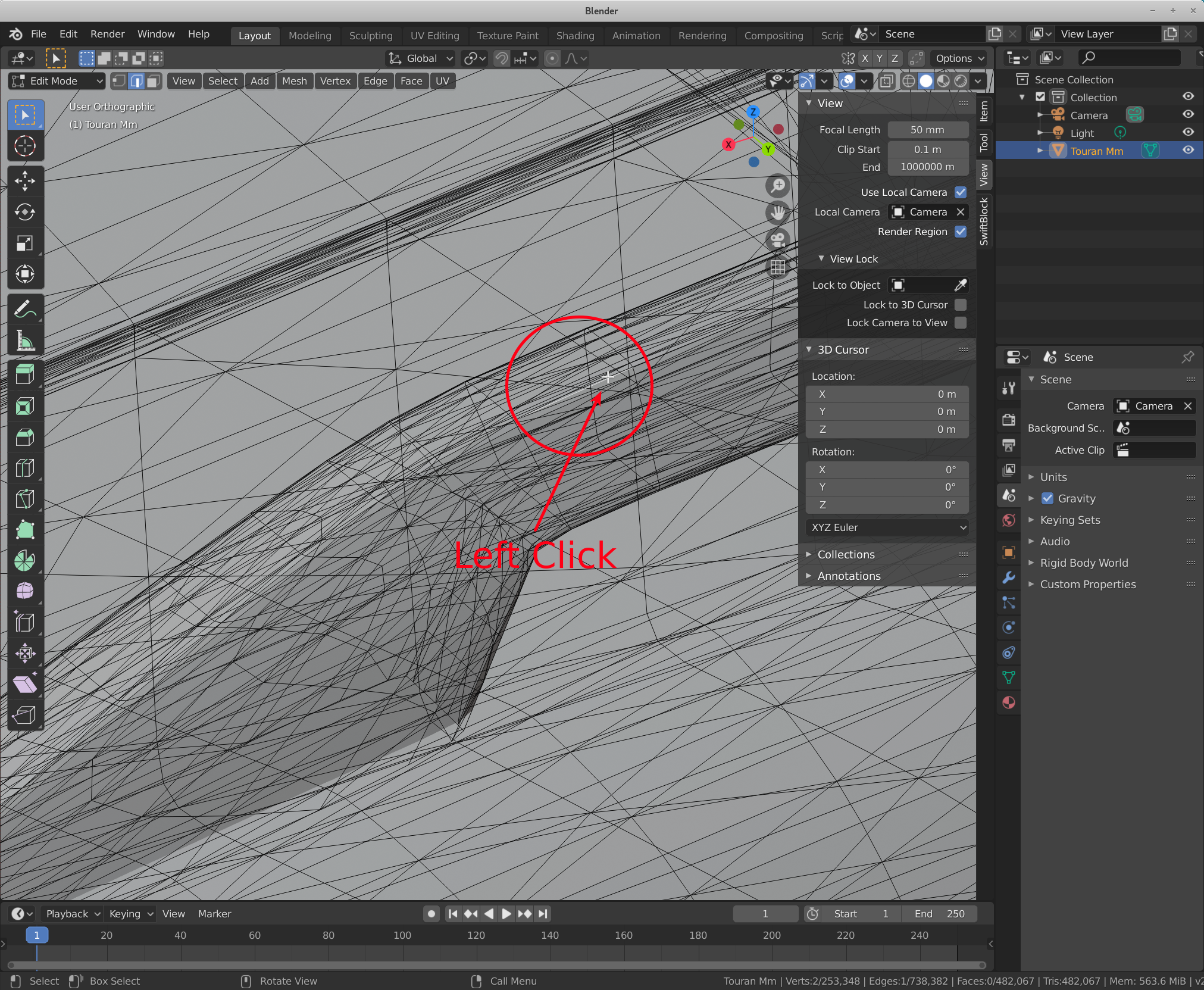 {width=”75%”}
 -
select another edge on the feature line: zoom to the next location and press Ctrl + Left click
The shortest path from the last selected edge and the current clicked edge will be added to the selection. To select edges as precise as possible, it might be required to click a number of intermediate locations. If a mistake is made, the last step can be undone by typing Ctrl+Z.
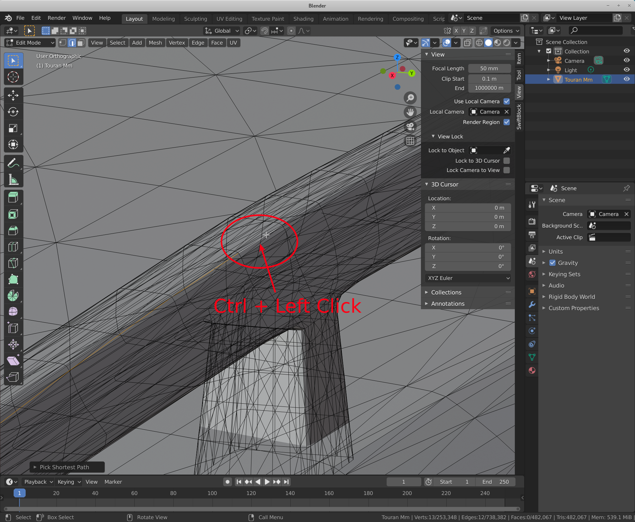 {width=”75%”}
 -
repeat the last step until the end of the feature line is reached.
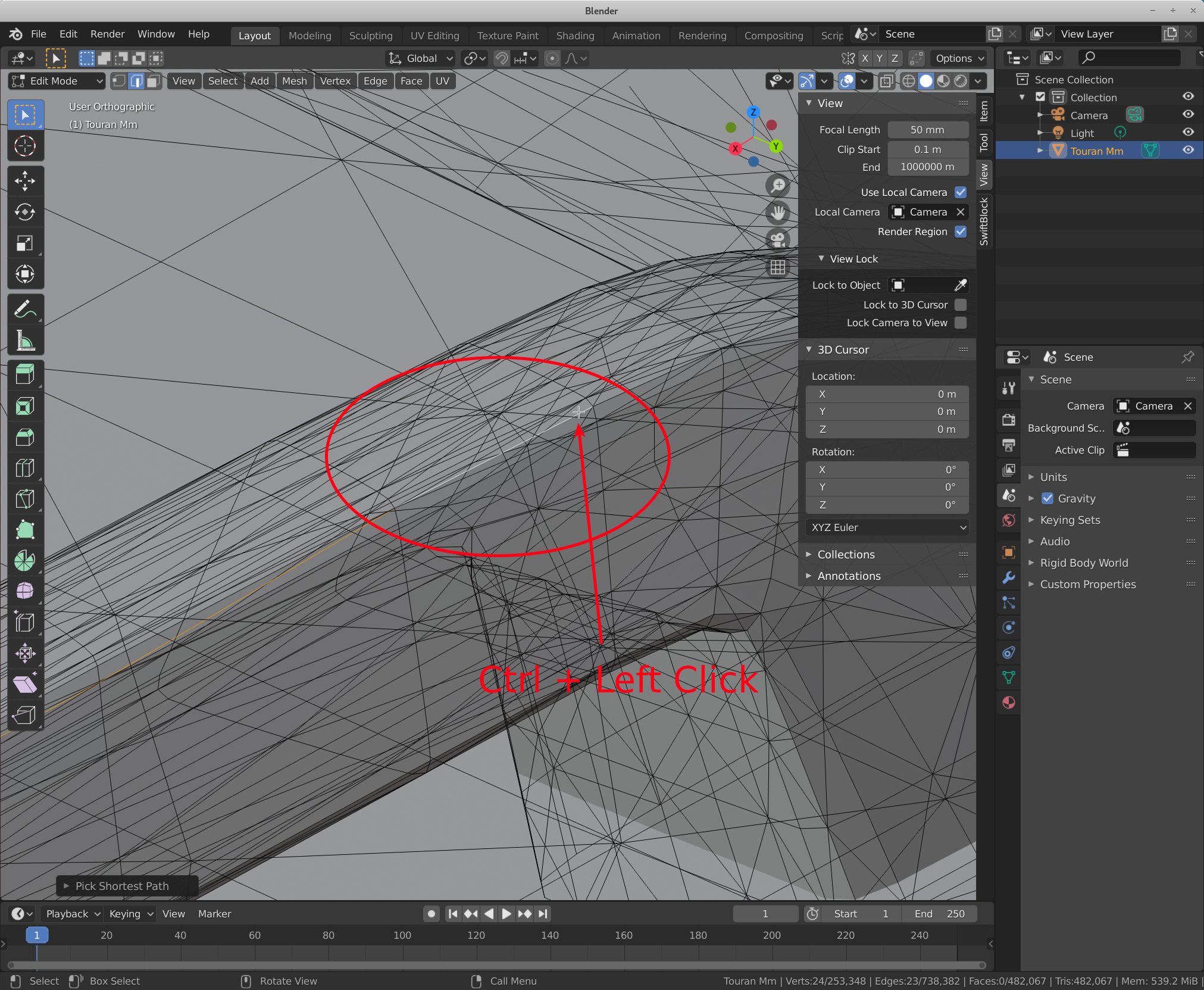 {width=”75%”}
 -
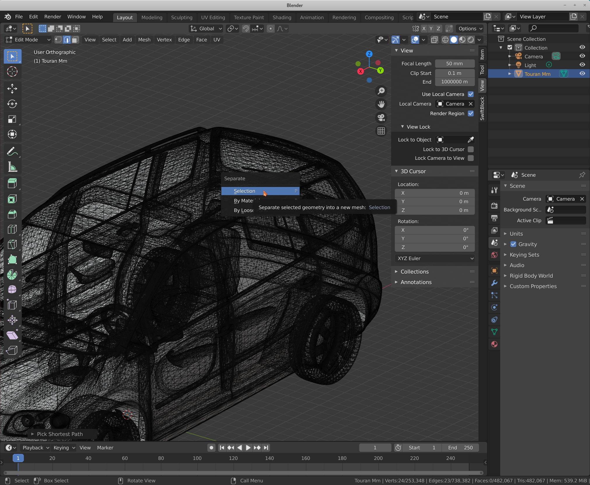
next create a new object from the selected edges by typing the key “P”.
Then select “Selection” to create the new part from the current selection.
Once the selection is split off, another chain of edges can be selected by repeating the steps from [pt:begin_sel].
 {width=”75%”}
 -
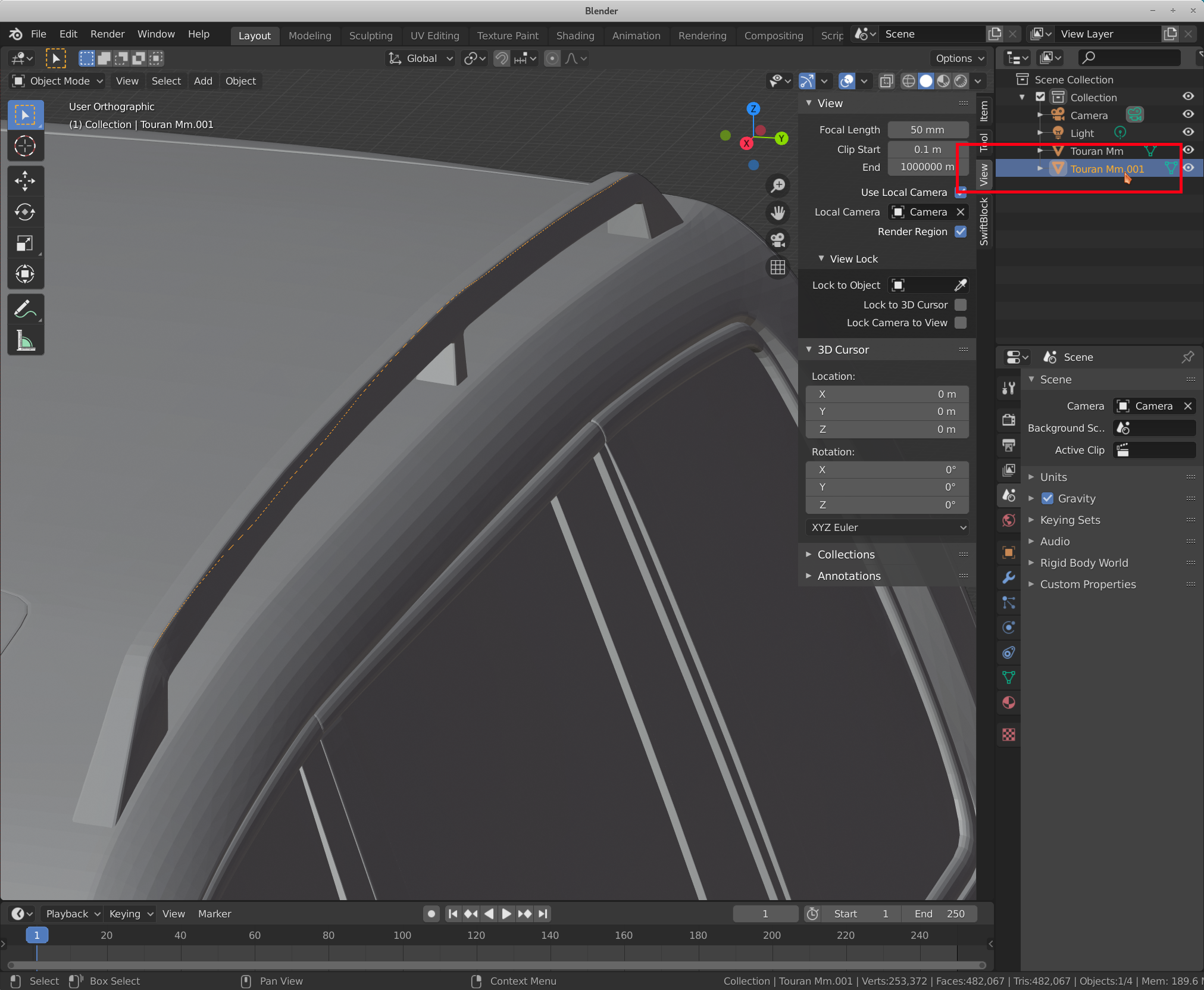
switch back to “Object Mode”
either by pressing the Tab key or by selecting “Object Mode” in the combo box in the upper left corner.
When multiple lines had been split into multiple new objects, these should be joined into a single one. To do so, select the objects in the object browser (upper right), then type “Ctrl+J”.
Note: the mouse should be over the 3D viewport for Blender to accept the keyboard shortcut.
 {width=”75%”}
 -
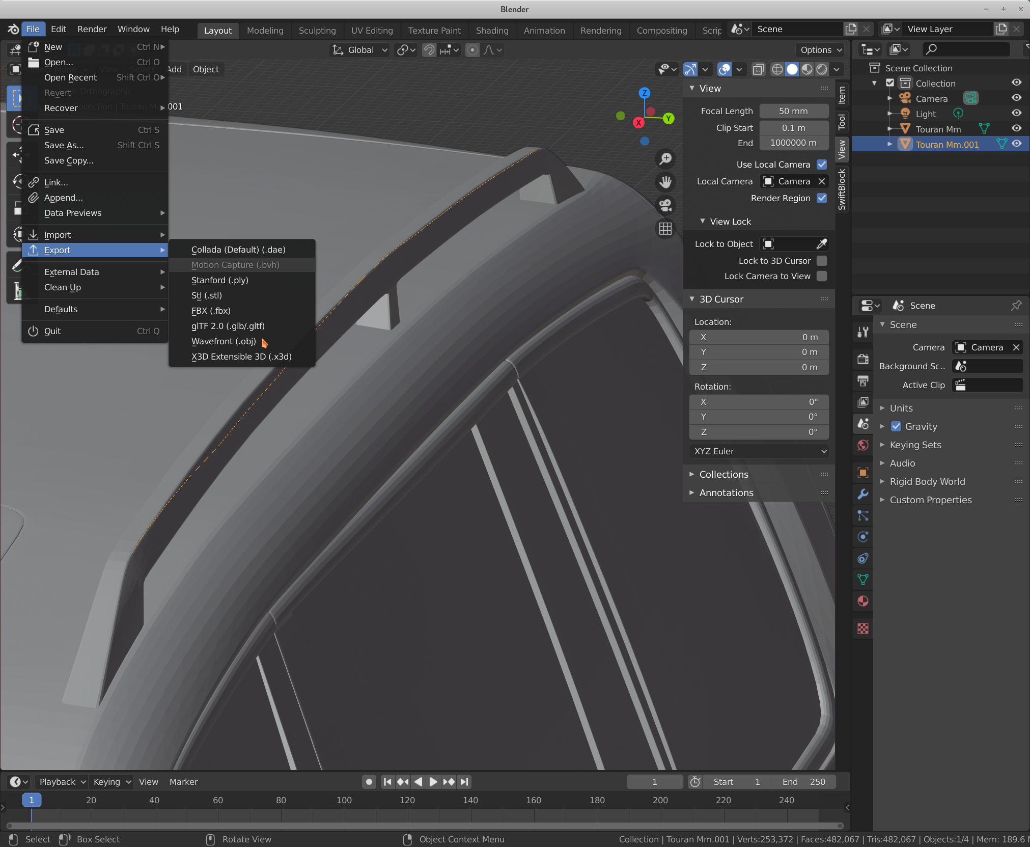
export the edges into an OBJ file.
Select the object in the object browser with a left click.
Then open the menu .
 {width=”75%”}
 -
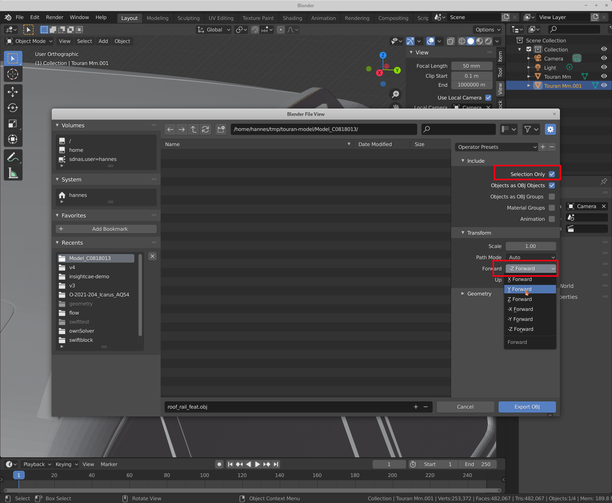
check the export settings. Make sure, the following is set:
-
“Selection only” is checked
(Otherwise also the surface will be included in the exported file)
-
In “Transform”, “Forward” is set to “Y Forward”
(Otherwise the geometry will be wrongly oriented after export)
 {width=”75%”}
 -
-
the resulting OBJ files can be loaded into Paraview and checked
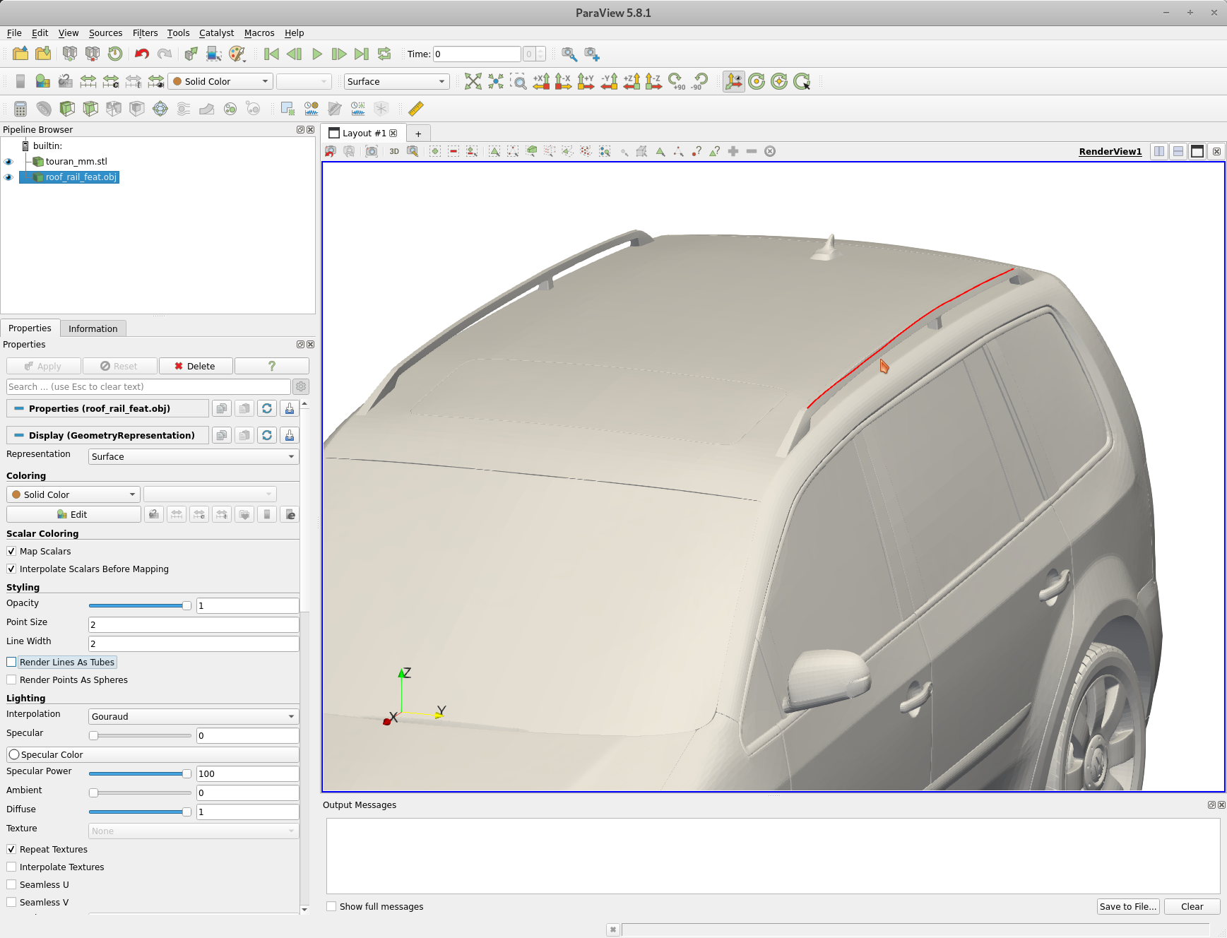 {width=”75%”}
 -
Finally, the OBJ files can be converted into OpenFOAM’s eMesh format. There is a tool called “surfaceFeatureConvert” in the OpenFOAM toolbox, which can perform this task. The file type is recognized from the extension. If not already done, the OpenFOAM environment needs to be loaded (here using the alias of1806):
$ of1806 $ surfaceFeatureConvert roof_rail_feat.obj roof_rail_feat.eMesh